Chapter 5 Non-Parametric Tests and Applications Using R
By the end of this chapter, you will be able to:
- Select the correct non-parametric test given the data structure, number of groups, and pairing status
- Implement the Sign test and Wilcoxon Signed-Rank test for one-sample and paired data
- Apply the Mann-Whitney U test to compare two independent groups
- Conduct Kruskal-Wallis ANOVA and appropriate post-hoc tests for 3+ independent groups
- Run the Friedman test for repeated-measures or blocked designs
- Report results in proper scientific writing format (APA / journal style)
Why this chapter? A clinical researcher studies pain reduction in 15 patients. Pain scores are on a 0–10 scale and are heavily skewed — the t-test’s normality assumption is clearly violated. Non-parametric tests solve this: they work on ranks instead of raw values, require no distributional assumptions, and remain valid for small samples. This chapter gives you the complete toolkit for distribution-free inference.
- Chapters 2 & 3: Descriptive statistics and confidence intervals
- Hypothesis testing: p-values, null/alternative hypotheses, Type I and II errors
- Chapter 3: Shapiro-Wilk test for normality (introduced there)
This final chapter covers the classic non-parametric hypothesis tests — the rank-and-sign-based alternatives to the t-test and ANOVA family, used when normality assumptions don’t hold or sample sizes are small.
This chapter uses course_dataset for most examples, exam_pairs (a small pre/post exam-score dataset) for the paired-test section, and the built-in datasets PlantGrowth, ToothGrowth, and sleep to show the same tests applied to completely different research questions.
5.1 Motivation, Advantages, and Limitations
Advantages: no distributional assumption required; robust to outliers and skew; valid for small samples; work directly on ranks or signs rather than raw values.
Limitations: generally less statistically powerful than the parametric equivalent when the parametric assumptions genuinely hold; hypotheses are framed around medians/distributions/ranks rather than means, which changes how you word your conclusions; fewer options exist for complex, multi-factor designs.
Non-Parametric Test Selection Matrix
Use this matrix to identify the correct test and R implementation based on your data structure:
| Scenario / Design | Dependent Var Type | Independent Var / Groups | Parametric Equivalent | Non-Parametric Test | R Implementation |
|---|---|---|---|---|---|
| One Sample (Proportion) | Binary / Categorical | None (compared to constant) | One-sample \(z\)-test | Binomial Test | binom.test(x, n, p) |
| One Sample (Median) | Continuous / Ordinal | None (compared to constant) | One-sample \(t\)-test | Sign Test | Custom function / binomial |
| Two Independent Groups | Continuous / Ordinal | Binary (2 independent groups) | Independent \(t\)-test | Mann-Whitney U / Wilcoxon Rank-Sum | wilcox.test(y ~ group) |
| Two Paired Measurements | Continuous / Ordinal | Paired / Repeated (2 related measurements) | Paired \(t\)-test | Wilcoxon Signed-Rank | wilcox.test(x, y, paired = TRUE) |
| Three+ Independent Groups | Continuous / Ordinal | Multiclass (3+ independent groups) | One-way ANOVA | Kruskal-Wallis | kruskal.test(y ~ group) |
| Three+ Repeated Measures | Continuous / Ordinal | Multiclass (3+ related measurements) | Repeated measures ANOVA | Friedman Test | friedman.test(y ~ time | id) |
Checking normality with the Shapiro-Wilk test is a common first step:
#>
#> Shapiro-Wilk normality test
#>
#> data: course_df$baseline_pain
#> W = 0.96216, p-value = 8.788e-05#>
#> Shapiro-Wilk normality test
#>
#> data: course_df$week8_pain
#> W = 0.95497, p-value = 1.665e-05Both p-values are well below 0.05, meaning we reject the assumption of normality — non-parametric methods are the safer choice for this variable.
5.2 One-Sample Tests
5.2.1 Binomial test — for a proportion against a hypothesized value
n_responders <- sum(course_df$response == "Responder")
n_total <- nrow(course_df)
binom.test(n_responders, n_total, p = 0.5)#>
#> Exact binomial test
#>
#> data: n_responders and n_total
#> number of successes = 131, number of trials = 180, p-value = 8.018e-10
#> alternative hypothesis: true probability of success is not equal to 0.5
#> 95 percent confidence interval:
#> 0.6565617 0.7913269
#> sample estimates:
#> probability of success
#> 0.7277778This tests whether the true response rate differs from a hypothesized 50%.
5.2.2 Sign test — for a median against a hypothesized value
The BSDA package provides SIGN.test() directly, but the sign test is simple enough to build from a single insight: it’s just a binomial test on the count of values above vs. below the hypothesized median.
Check Before You Run This (One-Sample Sign Test Diagnostics) Before running a Sign Test:
- Ordinal or Continuous Variable: The dependent variable should be measured on an ordinal or continuous scale.
- Independence: Observations must be independent of one another.
- No Distributional Assumptions: Unlike the Wilcoxon signed-rank test, the Sign Test does not assume that the distribution is symmetric around the median, making it the most robust test of all.
manual_sign_test <- function(x, mu = 0) {
diffs <- x - mu
diffs <- diffs[diffs != 0] # ties are dropped
n_pos <- sum(diffs > 0)
binom.test(n_pos, length(diffs), p = 0.5)
}
manual_sign_test(course_df$week8_pain, mu = 4)#>
#> Exact binomial test
#>
#> data: n_pos and length(diffs)
#> number of successes = 63, number of trials = 179, p-value = 9.116e-05
#> alternative hypothesis: true probability of success is not equal to 0.5
#> 95 percent confidence interval:
#> 0.2821879 0.4267169
#> sample estimates:
#> probability of success
#> 0.3519553The sign test only uses the direction (sign) of each deviation from the hypothesized value, throwing away information about magnitude. This makes it extremely robust — but also less powerful than a test that uses ranks, like the Wilcoxon signed-rank test coming up next.
How to Report This in a Paper: > “A one-sample sign test was conducted to determine if the median week-8 pain score differed from a clinical threshold of 4.0. The test indicated that the median pain score (Mdn = 3.1) was statistically significantly lower than 4.0, \(p < .001\) (\(n_{\text{above}} = 63, n_{\text{below}} = 116\)).”
Second example — built-in sleep dataset:
#>
#> Exact binomial test
#>
#> data: n_pos and length(diffs)
#> number of successes = 5, number of trials = 9, p-value = 1
#> alternative hypothesis: true probability of success is not equal to 0.5
#> 95 percent confidence interval:
#> 0.2120085 0.8630043
#> sample estimates:
#> probability of success
#> 0.5555556Using PlantGrowth$weight (built into R), test whether the median plant weight differs from a hypothesized value of 5.0, using both manual_sign_test() and binom.test() directly — confirm you get identical results.
5.3 Two Independent Groups: Mann-Whitney U (Wilcoxon Rank-Sum)
The Mann-Whitney U Test (also known as the Wilcoxon Rank-Sum Test) compares the distributions of two independent groups. It is the non-parametric alternative to the independent two-sample t-test.
Check Before You Run This (Mann-Whitney U Diagnostics) Before running a Mann-Whitney U test, verify these assumptions:
- Ordinal or Continuous Dependent Variable: The outcome variable must be ordinal or continuous.
- Independent Groups: The independent variable must consist of two categorical, independent groups.
- Independence of Observations: Observations within and between groups must be independent.
- Null Hypothesis (\(H_0\)): The distributions of the two groups are equal.
- Alternative Hypothesis (\(H_1\)): The distributions of the two groups are not equal.
5.3.1 How Rank-Sum Testing Works (The Logic of Ranks)
Instead of comparing means, this test ranks all observations from both groups combined from smallest to largest. Let’s see how this works on a tiny dummy dataset:
Dummy Example: * Group A:
c(5, 12)* Group B:c(3, 8)
- Combine and Sort: The combined dataset sorted is
c(3, 5, 8, 12).- Assign Ranks:
- Value
3(Group B) \(\rightarrow\) Rank 1- Value
5(Group A) \(\rightarrow\) Rank 2- Value
8(Group B) \(\rightarrow\) Rank 3- Value
12(Group A) \(\rightarrow\) Rank 4- Sum Ranks for each group:
- Sum for Group A (\(R_1\)): \(2 + 4 = 6\)
- Sum for Group B (\(R_2\)): \(1 + 3 = 4\)
If the rank sums are very different, it suggests one group systematically has larger values than the other.
5.3.2 Step-by-Step R Execution
Let’s run this test on our course_df comparing week 8 pain levels between the Treatment and Control groups:
# Run the test using formula notation: numeric_variable ~ grouping_variable
wilcox_result <- wilcox.test(week8_pain ~ treatment, data = course_df)
print(wilcox_result)#>
#> Wilcoxon rank sum test with continuity correction
#>
#> data: week8_pain by treatment
#> W = 2201, p-value = 1.499e-07
#> alternative hypothesis: true location shift is not equal to 05.3.3 Understanding the Output
W(Test Statistic): This is calculated from the sum of ranks of the first group.p-value: Here, \(p = 1.50 \times 10^{-7}\), which is extremely small and well below the \(0.05\) significance threshold. We reject the null hypothesis and conclude that week 8 pain levels differ significantly between the Treatment and Control groups.- Warning (“cannot compute exact p-value with ties”): R typically displays a warning message in the console when ties are present because it cannot compute the mathematically exact distribution (since multiple patients reported the same pain score, like two patients having a score of 3). R automatically splits ranks for tied values (giving them the average rank) and uses a normal approximation. This warning is expected and normal for datasets with integer or rounded scores.
The Math Behind It: Manual Mann-Whitney U Calculation The U statistic for the first group is calculated as: \[U_1 = R_1 - \frac{n_1(n_1 + 1)}{2}\] where \(R_1\) is the sum of ranks for Group 1, and \(n_1\) is its sample size.
For large samples, the distribution of \(U\) closely approximates a normal distribution. Under the null hypothesis, the mean (\(\mu_U\)) and standard error (\(\sigma_U\)) of \(U\) are: \[\mu_U = \frac{n_1 n_2}{2}, \quad \sigma_U = \sqrt{\frac{n_1 n_2(n_1 + n_2 + 1)}{12}}\] The test statistic is converted to a \(Z\)-score: \[Z = \frac{U_1 - \mu_U}{\sigma_U}\]
Let’s compute this manually in R to verify it matches R’s output:
# 1. Extract groups
g1 <- course_df$week8_pain[course_df$treatment == "New"]
g2 <- course_df$week8_pain[course_df$treatment == "Standard"]
n1 <- length(g1)
n2 <- length(g2)
# 2. Combine and rank
all_ranks <- rank(c(g1, g2))
r1 <- sum(all_ranks[1:n1])
# 3. Calculate U statistic (matches W exactly)
u1 <- r1 - n1 * (n1 + 1) / 2
u1#> [1] 2201# 4. Z normal approximation
mu_u <- (n1 * n2) / 2
sigma_u <- sqrt((n1 * n2 * (n1 + n2 + 1)) / 12)
z_score <- (u1 - mu_u) / sigma_u
z_score#> [1] -5.250062#> [1] 1.520481e-07Our manual \(U_1\) matches R’s \(W\) (\(2201\)) exactly! The manual p-value (\(1.52 \times 10^{-7}\)) is extremely close to R’s output (\(1.50 \times 10^{-7}\)). The minor difference is because R’s wilcox.test() adjusts the standard error (\(\sigma_U\)) to account for ties in the data and applies a continuity correction of \(0.5\) by default.
How to Report This in a Paper: > “A Mann-Whitney U test indicated that week 8 pain scores were statistically significantly lower in the New Treatment group (\(Mdn = 2.4\), \(n = 96\)) compared to the Standard Treatment group (\(Mdn = 4.3\), \(n = 84\)), \(W = 2201\), \(p < .001\). The effect size, calculated as rank-biserial correlation, was \(r = 1 - \frac{2W}{n_1 n_2} = 1 - \frac{2(2201)}{96 \times 84} = 0.45\), representing a moderate-to-strong effect.”
5.3.4 Second Example: Using ToothGrowth (Built-in)
Let’s compare tooth length (len) by supplement type (supp: orange juice OJ vs ascorbic acid VC):
#>
#> Wilcoxon rank sum exact test
#>
#> data: len by supp
#> W = 575.5, p-value = 0.06366
#> alternative hypothesis: true location shift is not equal to 05.3.5 Third Example: Subsetting Groups
If a dataset has 3 groups (e.g., control, treatment 1, treatment 2) and we only want to compare two, we must subset it first:
# Subset control and treatment 2 from PlantGrowth
pg_subset <- subset(PlantGrowth, group %in% c("ctrl", "trt2"))
# Run the test
wilcox.test(weight ~ group, data = pg_subset)#>
#> Wilcoxon rank sum exact test
#>
#> data: weight by group
#> W = 25, p-value = 0.06301
#> alternative hypothesis: true location shift is not equal to 0Exercise: Mann-Whitney U
- Load
course_dataset.csv. - Subset the data to compare
week8_painbetween Site A and Site B only. - Run the Wilcoxon Rank-Sum test and state your statistical conclusion.
5.4 Paired Measurements: Wilcoxon Signed-Rank Test
The Wilcoxon Signed-Rank Test is used to compare two related samples, matched samples, or repeated measurements on a single sample to assess whether their population mean ranks differ. It is the non-parametric alternative to the paired-samples t-test.
Check Before You Run This (Wilcoxon Signed-Rank Diagnostics) Before running a Wilcoxon Signed-Rank test, verify these assumptions:
- Ordinal or Continuous Dependent Variable: The paired variables must be ordinal or continuous.
- Paired/Matched Observations: Each subject must have exactly two paired measurements (e.g., pre-test vs. post-test).
- Symmetric Differences: The distribution of differences between the two paired groups should be approximately symmetric around the median of differences.
The Math Behind It: Wilcoxon Signed-Rank Test Let \(D_i = X_{1,i} - X_{2,i}\) be the differences between the paired observations.
- Exclude differences that are zero (\(D_i = 0\)).
- Rank the absolute differences \(|D_i|\) from smallest to largest, assigning average ranks to ties.
- Sum the ranks of the positive differences (\(W^+\)) and the negative differences (\(W^-\)).
- The test statistic \(W\) (in R, printed as \(V\)) is: \[V = \sum_{D_i > 0} \text{Rank}(|D_i|)\] For large samples, the test statistic \(V\) is converted to a \(Z\)-score using the mean and standard error of the signed-rank distribution.
This section switches to exam_pairs — 25 students with a pre-test and post-test score — a cleaner example of genuinely paired data than repeating the pain-score columns again.
wilcox_paired <- wilcox.test(exam_df$pre_test, exam_df$post_test, paired = TRUE)
print(wilcox_paired)#>
#> Wilcoxon signed rank exact test
#>
#> data: exam_df$pre_test and exam_df$post_test
#> V = 8.5, p-value = 1.55e-06
#> alternative hypothesis: true location shift is not equal to 0How to Report This in a Paper: > “A Wilcoxon signed-rank test was conducted to compare exam performance before and after the tutorial. The test indicated that student scores were statistically significantly higher after the tutorial (\(Mdn = 71\)) compared to before the tutorial (\(Mdn = 61\)), \(V = 8.5\), \(p < .001\), indicating a strong positive effect of the intervention.”
A very common mistake: running the unpaired version of this test (wilcox.test(pre_test, post_test) without paired = TRUE) on data that’s actually paired. This throws away the pairing information — the fact that the same student appears in both columns — and can give a misleading result. Always ask: are these the same subjects measured twice, or two different independent groups?
Second example — with the course dataset’s baseline vs. week 8 pain:
#>
#> Wilcoxon signed rank test with continuity correction
#>
#> data: course_df$baseline_pain and course_df$week8_pain
#> V = 15820, p-value < 2.2e-16
#> alternative hypothesis: true location shift is not equal to 0Using exam_df, also run the unpaired version of the same test by mistake (wilcox.test(exam_df$pre_test, exam_df$post_test), no paired = TRUE). Compare the p-value to the correct paired version above — how different is the conclusion?
5.5 Three or More Independent Groups: Kruskal-Wallis
The Kruskal-Wallis Test is a rank-based non-parametric test that can be used to determine if there are statistically significant differences between three or more groups on an ordinal or continuous dependent variable. It is the non-parametric alternative to the one-way ANOVA.
Check Before You Run This (Kruskal-Wallis Diagnostics) Before running a Kruskal-Wallis test, verify these assumptions:
- Ordinal or Continuous Dependent Variable: The outcome variable must be ordinal or continuous.
- Independent Groups: The independent grouping variable must contain 3 or more categorical, independent groups.
- Independence of Observations: Observations within and between groups must be independent.
The Math Behind It: Kruskal-Wallis H Test Like other rank tests, observations from all groups are combined and ranked. The test statistic \(H\) is computed as: \[H = \frac{12}{N(N+1)} \sum_{j=1}^{k} \frac{R_j^2}{n_j} - 3(N+1)\] where:
- \(k\) is the number of groups.
- \(n_j\) is the sample size of group \(j\).
- \(N\) is the total sample size across all groups (\(N = \sum n_j\)).
- \(R_j\) is the sum of ranks for group \(j\).
Under the null hypothesis, \(H\) follows a Chi-Square (\(\chi^2\)) distribution with \(k-1\) degrees of freedom. The p-value is computed in R using pchisq(H, df = k - 1, lower.tail = FALSE).
#>
#> Kruskal-Wallis rank sum test
#>
#> data: week8_pain by site
#> Kruskal-Wallis chi-squared = 1.5744, df = 2, p-value = 0.4551A significant result tells you at least one site differs from the others — but not which one(s). Follow up with pairwise comparisons and a multiple-comparison correction:
#>
#> Pairwise comparisons using Wilcoxon rank sum test with continuity correction
#>
#> data: course_df$week8_pain and course_df$site
#>
#> Site A Site B
#> Site B 0.78 -
#> Site C 0.94 1.00
#>
#> P value adjustment method: bonferroniWhy the correction matters: if you ran many pairwise tests at the usual 0.05 threshold without any adjustment, you’d accumulate a much higher chance of at least one false positive purely by chance. The Bonferroni correction (dividing your significance threshold by the number of comparisons) is a simple, conservative way to control that risk.
How to Report This in a Paper: > “A Kruskal-Wallis test showed no statistically significant difference in week 8 pain levels across the three hospital sites, \(H(2) = 1.57\), \(p = .455\). The median pain scores were \(3.40\) for Site A, \(2.85\) for Site B, and \(3.00\) for Site C. Consistent with the overall test, post-hoc pairwise Wilcoxon rank-sum tests with Bonferroni correction showed no significant differences between any pair of sites (all adjusted \(p \ge .78\)).”
Second example — PlantGrowth, all three groups:
#>
#> Kruskal-Wallis rank sum test
#>
#> data: weight by group
#> Kruskal-Wallis chi-squared = 7.9882, df = 2, p-value = 0.01842#>
#> Pairwise comparisons using Wilcoxon rank sum exact test
#>
#> data: PlantGrowth$weight and PlantGrowth$group
#>
#> ctrl trt1
#> trt1 0.590 -
#> trt2 0.189 0.027
#>
#> P value adjustment method: bonferroniRun kruskal.test() on course_df$baseline_pain grouped by activity_level (Low/Moderate/High). Is there a significant difference? If so, which pairs differ?
5.6 Repeated Measures on the Same Subjects: The Friedman Test
The Friedman Test is the non-parametric version of the one-way repeated measures ANOVA. It is used when the same subjects are measured three or more times under different conditions (or at different time points).
Check Before You Run This (Friedman Test Diagnostics) Before running a Friedman test, verify these assumptions:
- Ordinal or Continuous Dependent Variable: The outcome variable must be ordinal or continuous.
- Repeated Measures / Blocks: One group of subjects is measured on 3 or more occasions (or matched blocks).
- No Missing Data: The test requires a complete block design. If a subject is missing a score at any time point, R will throw an error or exclude the subject.
The Math Behind It: Friedman Q Test For each subject (or block), the \(k\) measurements are ranked from \(1\) to \(k\). The test statistic \(Q\) is: \[Q = \frac{12}{n k (k+1)} \sum_{j=1}^{k} R_j^2 - 3n(k+1)\] where:
- \(n\) is the number of subjects (blocks).
- \(k\) is the number of repeated measurements (groups).
- \(R_j\) is the sum of ranks for treatment/time point \(j\).
Under the null hypothesis, \(Q\) follows a Chi-Square (\(\chi^2\)) distribution with \(k-1\) degrees of freedom.
- Null Hypothesis (\(H_0\)): The distributions (medians) across all time points are equal.
- Alternative Hypothesis (\(H_1\)): At least one time point distribution differs from the others.
5.6.1 Step 1: Reshaping Wide Data to Long Format
In our course_df dataset, the pain scores for each patient are stored in three separate columns: baseline_pain, week4_pain, and week8_pain (wide format).
To run the Friedman test, R requires the data to be in long format (where each observation is its own row, with a subject ID, a time point label, and the score).
Let’s use tidyr::pivot_longer() (which you learned in Chapter 2!) to reshape the data:
library(tidyr)
library(dplyr)
# 1. Select the relevant columns to see the wide structure:
course_df %>%
select(id, baseline_pain, week4_pain, week8_pain) %>%
head(3)# 2. Pivot the pain columns into long format:
long_pain <- course_df %>%
select(id, baseline_pain, week4_pain, week8_pain) %>%
pivot_longer(
cols = c(baseline_pain, week4_pain, week8_pain),
names_to = "time",
values_to = "pain"
)
# 3. View the reshaped long structure:
head(long_pain, 6)5.6.2 Step 2: Running the Friedman Test
Now that the data is in long format, we can run friedman.test():
# Formula: value_variable ~ grouping_variable | subject_id
friedman_result <- friedman.test(pain ~ time | id, data = long_pain)
print(friedman_result)#>
#> Friedman rank sum test
#>
#> data: pain and time and id
#> Friedman chi-squared = 264.98, df = 2, p-value < 2.2e-165.6.3 Understanding the Output
Friedman chi-squared: The test statistic.p-value: Here, \(p < 2.2 \times 10^{-16}\) (extremely small). We reject the null hypothesis and conclude that pain scores differ significantly across the three time points.
How to Report This in a Paper: > “A Friedman test indicated that pain levels differed statistically significantly across the three time points (baseline, week 4, week 8), \(\chi^2(2) = 264.98\), \(p < .001\) (\(\text{Kendall's W effect size } = Q / (n(k-1)) = 0.74\), representing a moderate-to-strong effect). Post-hoc pairwise Wilcoxon signed-rank tests with Bonferroni correction showed a statistically significant reduction in pain scores at every step (all adjusted \(p < .001\)).”
5.6.4 Step 3: Post-Hoc Pairwise Comparisons
Just like the Kruskal-Wallis test, the Friedman test only tells us that at least one time point differs. To find out which specific time points are different, we perform pairwise Wilcoxon signed-rank tests with a Bonferroni correction:
# Run pairwise paired Wilcoxon tests
pairwise_results <- pairwise.wilcox.test(
x = long_pain$pain,
g = long_pain$time,
paired = TRUE,
p.adjust.method = "bonferroni"
)
print(pairwise_results)#>
#> Pairwise comparisons using Wilcoxon signed rank test with continuity correction
#>
#> data: long_pain$pain and long_pain$time
#>
#> baseline_pain week4_pain
#> week4_pain <2e-16 -
#> week8_pain <2e-16 <2e-16
#>
#> P value adjustment method: bonferroni5.6.5 Understanding Post-Hoc Output
The table lists adjusted p-values for each comparison:
week4_painvsbaseline_pain: \(p < 0.001\) (Significant)week8_painvsbaseline_pain: \(p < 0.001\) (Significant)week8_painvsweek4_pain: \(p < 0.001\) (Significant)
We conclude that pain scores decrease significantly at each subsequent follow-up interval.
The dedicated post-hoc test for Friedman is the Nemenyi test, available via PMCMRplus::frdAllPairsNemenyiTest(). The pairwise Wilcoxon approach shown above is a widely-used approximation when that package is not installed.
Exercise: Friedman Post-Hoc Interpretation Verify the pairwise output on your own console. Explain in your own words why we need a “Bonferroni adjustment” when running multiple pairwise tests.
5.7 Capstone: Selecting, Justifying, Running, and Reporting a Test
Let’s work through a complete example end to end, exactly as you’ll be asked to do in the lab.
Research question: “Is there a difference in week4_pain across the three sites?”
# STEP 1: Identify the design
# Three independent groups (Site A, B, C) ->
# candidates are one-way ANOVA or Kruskal-Wallis
# STEP 2: Check assumptions
tapply(course_df$week4_pain, course_df$site, shapiro.test)#> $`Site A`
#>
#> Shapiro-Wilk normality test
#>
#> data: X[[i]]
#> W = 0.974, p-value = 0.2025
#>
#>
#> $`Site B`
#>
#> Shapiro-Wilk normality test
#>
#> data: X[[i]]
#> W = 0.97897, p-value = 0.254
#>
#>
#> $`Site C`
#>
#> Shapiro-Wilk normality test
#>
#> data: X[[i]]
#> W = 0.97421, p-value = 0.4369# STEP 3: Select the test
# At least one group shows meaningful non-normality ->
# Kruskal-Wallis is the safer choice
# STEP 4: Run and extract results
kw_result <- kruskal.test(week4_pain ~ site, data = course_df)
kw_result#>
#> Kruskal-Wallis rank sum test
#>
#> data: week4_pain by site
#> Kruskal-Wallis chi-squared = 1.3809, df = 2, p-value = 0.5014# STEP 5: Post-hoc if needed
if (kw_result$p.value < 0.05) {
print(pairwise.wilcox.test(
course_df$week4_pain,
course_df$site,
p.adjust.method = "bonferroni"
))
}# STEP 6: Report in plain language
cat(sprintf(
paste0(
"A Kruskal-Wallis test found %s evidence of alpha difference in ",
"week-4 pain scores across the three sites (H = %.2f, p = %.3f).\n"
),
ifelse(
kw_result$p.value < 0.05,
"statistically significant",
"no statistically significant"
),
kw_result$statistic,
kw_result$p.value
))#> A Kruskal-Wallis test found no statistically significant evidence of alpha difference in week-4 pain scores across the three sites (H = 1.38, p = 0.501).Pick your own research question from course_dataset that this chapter hasn’t already answered (for example: “Does sex relate to response?” — careful, that one might actually need Chapter 4’s tools, not this chapter’s! — or “Is there a difference in age between responders and non-responders?”). Work through all six capstone steps yourself, ending with a one-paragraph plain-language write-up.
- Non-parametric tests trade some statistical power for robustness to non-normality and outliers.
- One-sample: binomial test (proportions) or sign test (medians) — the sign test is just a binomial test on the count of values above/below the hypothesized value.
- Two independent groups: Mann-Whitney U / Wilcoxon rank-sum, via
wilcox.test(y ~ group). - Two paired measurements: Wilcoxon signed-rank, via
wilcox.test(x, y, paired = TRUE)— always double check pairing is correct. - 3+ independent groups: Kruskal-Wallis, followed by pairwise Wilcoxon with a correction if significant.
- 3+ repeated measurements: Friedman test, using long-format data and a correctly specified
blocksterm. - A consistent six-step workflow (design → assumptions → test selection → run → post-hoc → plain-language report) will serve you well beyond this course.
Non-Parametric Scenario Bank (Practice Exercises)
Practice identifying the correct statistical test for each of the following research scenarios using the decision matrix from Section 5.1.1. (Note: These exercises focus on test selection and do not require code).
Scenario 1
A hospital administrator wants to compare the patient satisfaction ratings (measured on a 1-to-5 Likert scale) between Ward A (\(n = 45\)) and Ward B (\(n = 50\)). Satisfaction scores are highly skewed. * Answer: Mann-Whitney U / Wilcoxon Rank-Sum test (comparing two independent groups on ordinal data).
Scenario 2
A clinical researcher measures the pain levels (on a 0-to-10 visual analog scale) of 30 chronic pain patients at three distinct time points: baseline, month 1, and month 3. The pain scores violate normality assumptions at all time points. * Answer: Friedman Test (comparing three related measurements on the same subjects over time).
Scenario 3
A psychologist wants to test if the median score on a cognitive test in a sample of elderly adults (\(n = 18\)) is significantly different from the national average median of 70. The sample data shows severe outliers. * Answer: Sign Test (one-sample median test with no symmetry assumptions).
Scenario 4
A geneticist wants to compare the expression levels of a specific gene across five different mouse strains (8 mice per strain). The expression levels are highly non-normal. * Answer: Kruskal-Wallis test (comparing 3+ independent groups on continuous, non-normal data).
Scenario 5
A diagnostic study compares the classifications (“Mild”, “Moderate”, “Severe”) of 100 radiographs made by a resident doctor and an expert radiologist. The researcher wants to assess the level of agreement between the two. * Answer: Weighted Cohen’s Kappa (measuring agreement between two raters on ordinal classifications).
5.8 Where to Go From Here
You’ve now covered the full arc of this course: from R fundamentals, through descriptive statistics and programming, to resampling-based confidence intervals, categorical data analysis, and non-parametric hypothesis testing. The Appendix that follows documents every dataset used throughout this book in one place, for quick reference.
Chapter 5 covered:
- When to use non-parametric tests: Non-normal data, small samples (\(n < 20\)), ordinal outcomes, or when robustness to outliers is needed
- One-sample / paired tests:
- Sign test: Tests whether median equals a value; uses only the sign of differences → least powerful
- Wilcoxon Signed-Rank test: Uses ranks of absolute differences → more powerful than Sign test
- Two-sample tests:
- Mann-Whitney U (= Wilcoxon Rank-Sum): Compares medians / distributions of two independent groups
- Multi-group tests:
- Kruskal-Wallis: Non-parametric one-way ANOVA; significant result → follow with Dunn’s post-hoc test
- Friedman test: Non-parametric repeated-measures ANOVA; for blocked / matched designs
| Design | Parametric | Non-Parametric | R Function |
|---|---|---|---|
| 1 sample vs. constant | One-sample \(t\) | Sign / Wilcoxon SR | wilcox.test(x, mu=) |
| 2 independent groups | Independent \(t\) | Mann-Whitney U | wilcox.test(y ~ g) |
| 2 paired measurements | Paired \(t\) | Wilcoxon SR | wilcox.test(x,y,paired=TRUE) |
| 3+ independent groups | One-way ANOVA | Kruskal-Wallis | kruskal.test(y ~ g) |
| 3+ repeated measures | Repeated ANOVA | Friedman | friedman.test(y ~ t | id) |
Congratulations — you have completed the Statistical Computing and Non-Parametric Inference Using R course! You now have a complete toolkit: R programming (Ch.1), descriptive analysis (Ch.2), confidence intervals and the bootstrap (Ch.3), categorical data analysis (Ch.4), and distribution-free hypothesis testing (Ch.5).
5.9 Lab 5: Full Non-Parametric Workflow on the Course Dataset
Objective: Apply the complete non-parametric testing workflow — from normality checking through to post-hoc analysis and reporting — on a real dataset.
Datasets: course_dataset.csv and exam_pairs.csv
5.9.1 Step 1: Load Data and Check Normality
course_df <- read.csv("data/course_dataset.csv")
exam_df <- read.csv("data/exam_pairs.csv")
# Shapiro-Wilk test for baseline_pain
shapiro.test(course_df$baseline_pain)#>
#> Shapiro-Wilk normality test
#>
#> data: course_df$baseline_pain
#> W = 0.96216, p-value = 8.788e-05#>
#> Shapiro-Wilk normality test
#>
#> data: course_df$week8_pain
#> W = 0.95497, p-value = 1.665e-05# Visual check
par(mfrow = c(1, 2))
hist(course_df$baseline_pain, main = "Baseline Pain", col = "#AED6F1")
hist(course_df$week8_pain, main = "Week 8 Pain", col = "#A9DFBF")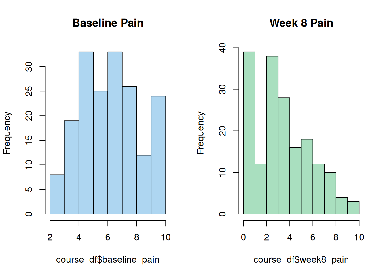
5.9.2 Step 2: Paired Analysis (Wilcoxon Signed-Rank)
# Did pain decrease from baseline to week 8?
wilcox.test(course_df$baseline_pain, course_df$week8_pain,
            paired = TRUE, alternative = "greater")
#>
#> Wilcoxon signed rank test with continuity correction
#>
#> data: course_df$baseline_pain and course_df$week8_pain
#> V = 15820, p-value < 2.2e-16
#> alternative hypothesis: true location shift is greater than 0Interpret: Report W statistic, p-value, and whether you reject \(H_0\).
5.9.3 Step 3: Two-Group Comparison (Mann-Whitney)
# Does baseline pain differ between treatment groups?
wilcox.test(baseline_pain ~ treatment, data = course_df)
#>
#> Wilcoxon rank sum test with continuity correction
#>
#> data: baseline_pain by treatment
#> W = 3863, p-value = 0.6288
#> alternative hypothesis: true location shift is not equal to 05.9.4 Step 4: Kruskal-Wallis for 3+ Groups
# Compare baseline pain across response categories
kruskal.test(baseline_pain ~ response, data = course_df)
#>
#> Kruskal-Wallis rank sum test
#>
#> data: baseline_pain by response
#> Kruskal-Wallis chi-squared = 15.065, df = 1, p-value = 0.0001039# Post-hoc (if significant)
if (kruskal.test(baseline_pain ~ response, data = course_df)$p.value < 0.05) {
library(PMCMRplus)
kwAllPairsDunnTest(baseline_pain ~ as.factor(response), data = course_df,
p.adjust.method = "bonferroni")
}#> Non-Responder
#> Responder 1e-045.9.5 Step 5: Write a Results Paragraph
Using the results above, write a 3–4 sentence results section in APA format, as you would in a journal paper. Include: the test used, the test statistic, degrees of freedom (if applicable), p-value, and a plain-English conclusion.
5.9.6 Lab Exercises
- Run the Sign test (manual binomial approach) on the paired pain data. Does the conclusion match the Wilcoxon Signed-Rank result? Why might they differ?
- Use the
exam_pairsdataset: run a Wilcoxon Signed-Rank test to check if exam scores improved from pre-test to post-test. - Compute the effect size \(r = Z / \sqrt{N}\) for the Mann-Whitney test in Step 3. Is the effect small, medium, or large (by Cohen’s conventions)?