A Answer Key Appendix (Instructor/TA Reference)
Solutions to every embedded exercise, organized by chapter/section. Written for you or a TA to grade against — not meant to be handed to students as-is, since several intentionally require interpretation, not just code.
A.1 Chapter 1
A.1.1 §1.2 Workspace management
#> [1] "course_df"     "exam_df"       "my_age"        "my_name"
#> [5] "scores" "used_r_before"#> [1] "course_df" "exam_df" "my_age" "my_name" "scores"#> [1] FALSEA.1.2 §1.3.4 Importing / str() comparison
scores_csv <- read.csv("data/student_scores.csv")
scores_txt <- read.table("data/student_scores.txt", header = TRUE, sep = "\t")
str(scores_txt)
#> 'data.frame': 40 obs. of 5 variables:
#> $ id : int 1 2 3 4 5 6 7 8 9 10 ...
#> $ name : chr "Student_01" "Student_02" "Student_03" "Student_04" ...
#> $ group : chr "A" "A" "A" "B" ...
#> $ score : int 63 66 49 89 69 95 92 69 77 92 ...
#> $ hours_studied: num 4.7 5.3 4.6 4.4 1.5 4.5 1.4 7.3 3 5.3 ...#> 'data.frame': 40 obs. of 5 variables:
#> $ id : int 1 2 3 4 5 6 7 8 9 10 ...
#> $ name : chr "Student_01" "Student_02" "Student_03" "Student_04" ...
#> $ group : chr "A" "A" "A" "B" ...
#> $ score : int 63 66 49 89 69 95 92 69 77 92 ...
#> $ hours_studied: num 4.7 5.3 4.6 4.4 1.5 4.5 1.4 7.3 3 5.3 ...Both group columns import as character, identical to the .csv version — read.table()/read.csv() don’t auto-convert strings to factors by default in modern R (stringsAsFactors = FALSE is the default since R 4.0).
A.1.4 §1.6 quarterly_sales array
quarterly_sales <- array(
  data = 1:24,
  dim = c(2, 3, 4),
  dimnames = list(
    c("ProductA", "ProductB"),
    c("RegionN", "RegionS", "RegionE"),
    c("Q1", "Q2", "Q3", "Q4")
  )
)
quarterly_sales["ProductB", "RegionE", ]           # all 4 quarters
#> Q1 Q2 Q3 Q4
#> 6 12 18 24#> [1] 40A.1.5 §1.9 List indexing
my_favorites <- list(
  movies = c("Inception", "Interstellar"),
  rating = 9.5
)
my_favorites$movies[2]          # "Interstellar"
#> [1] "Interstellar"#> [1] "list"#> [1] "character"Explanation: [1] keeps the train-car wrapper (still a list); [[1]] opens the car and returns the cargo directly (the character vector inside).
A.1.6 §1.10 Structure-matching discussion
- Monthly temperatures, one city, one year → vector (single type, 1D)
- Gradebook (names, scores, pass/fail) → data frame (mixed types)
- Sales: 5 products × 4 regions × 4 quarters → array (3D, single type)
- Blood type of 200 patients → factor (fixed categorical levels)
- Clustering output (assignments + centers + summary df) → list (heterogeneous bundle)
A.2 Chapter 2
A.2.1 §2.1 mtcars wt vs qsec
#> [1] 3.21725#> [1] 3.325#> [1] 17.84875#> [1] 17.71wt has the larger mean/median gap — a few heavy cars (e.g. Lincoln Continental, Chrysler Imperial) pull the mean up; qsec is comparatively symmetric.
A.2.2 §2.2 chickwts skewness
skewness_manual <- function(x) {
  n <- length(x)
  m <- mean(x)
  if (n < 3) return(NA)  # Handle edge cases
  (sum((x - m)^3) / n) / (sum((x - m)^2) / n)^(3/2)
}
skewness_manual(chickwts$weight)
#> [1] -0.01161035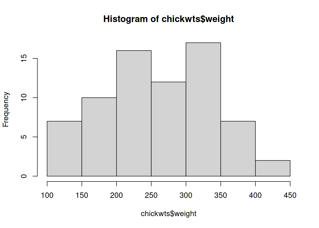 Result is close to 0 / essentially symmetric (very slightly left-skewed, -0.011) — roughly symmetric compared to
 airquality$Ozone’s skewness of ~1.2.
A.2.4 §2.4 even/odd loop
#> 1 odd
#> 2 even
#> 3 odd
#> 4 even
#> 5 odd
#> 6 even
#> 7 odd
#> 8 even
#> 9 odd
#> 10 even
A.3 Chapter 3
A.3.1 §3.5 course_dataset baseline_pain median CI
median_fn <- function(data, indices) median(data[indices])
boot_pain <- boot(
  course_df$baseline_pain,
  statistic = median_fn,
  R = 2000
)
boot.ci(boot_pain, type = "perc")
#> BOOTSTRAP CONFIDENCE INTERVAL CALCULATIONS
#> Based on 2000 bootstrap replicates
#>
#> CALL :
#> boot.ci(boot.out = boot_pain, type = "perc")
#>
#> Intervals :
#> Level Percentile
#> 95% ( 5.7, 6.6 )
#> Calculations and Intervals on Original Scale#> [1] 5.965246 6.583643
#> attr(,"conf.level")
#> [1] 0.95Talking point: baseline_pain is mildly skewed (right tail), so expect the bootstrap median CI and the t-based mean CI to tell a similar general story (both centered ~6–7) but not be numerically comparable, since one targets the median and the other the mean — a good moment to reinforce that these two CIs answer different questions, not competing versions of the same question.
A.3.2 §3.7 Repeat 5-step workflow for Standard group
mean_fn2 <- function(data, indices) mean(data[indices])
standard_pain <- course_df$week8_pain[course_df$treatment == "Standard"]
hist(standard_pain)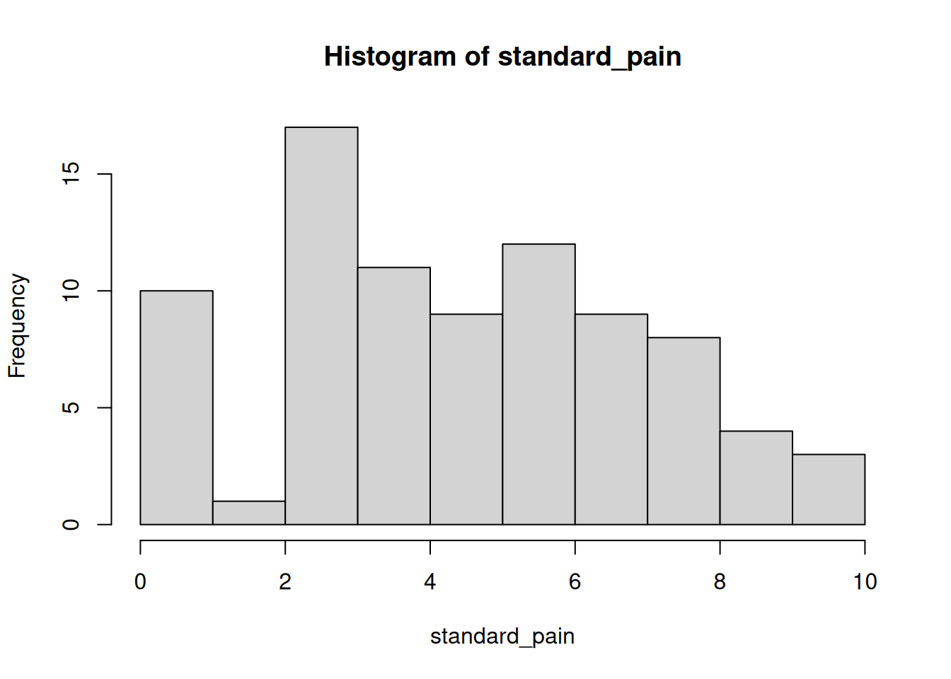
#>
#>  Shapiro-Wilk normality test
#>
#> data:  standard_pain
#> W = 0.97629, p-value = 0.1234
boot_standard <- boot(standard_pain, statistic = mean_fn2, R = 2000)
ci_standard <- boot.ci(boot_standard, type = "perc")
ci_standard#> BOOTSTRAP CONFIDENCE INTERVAL CALCULATIONS
#> Based on 2000 bootstrap replicates
#>
#> CALL :
#> boot.ci(boot.out = boot_standard, type = "perc")
#>
#> Intervals :
#> Level Percentile
#> 95% ( 3.966, 5.040 )
#> Calculations and Intervals on Original ScaleGrading point: the New-treatment CI (approx. 2.08-2.83) and the Standard-treatment CI should not overlap given the simulated effect sizes in the data generator — that non-overlap is what students should identify and state supports a real treatment difference (consistent with the Ch. 4/5 tests on the same outcome).
A.4 Chapter 4
A.4.1 §4.1 treatment × activity_level table
#>
#>            High Low Moderate
#>   New        24  39       33
#>   Standard   13  28       43
Read off the New/High cell directly from the printed table.
A.4.2 §4.2 InsectSprays exercise
InsectSprays$high_count <- ifelse(InsectSprays$count > 10, "High", "Low")
tab <- table(InsectSprays$spray, InsectSprays$high_count)
chisq.test(tab)$expected
#>
#> High Low
#> A 5.166667 6.833333
#> B 5.166667 6.833333
#> C 5.166667 6.833333
#> D 5.166667 6.833333
#> E 5.166667 6.833333
#> F 5.166667 6.833333With 6 spray types × 2 outcome levels and only 12 obs per spray, several expected counts will fall below 5 → use fisher.test(tab), not chi-square.
A.4.3 §4.3 Trend test p-value comparison
trend_tab <- table(course_df$activity_level, course_df$response)
chisq.test(trend_tab)$p.value        # generic association test
#> [1] 0.2193672The plain chi-square p-value will typically be larger (less significant) than the trend test’s, because it ignores the ordering of Low < Moderate < High and “spends” a degree of freedom testing a more general (less specific) alternative. Since activity level genuinely has a natural order, the trend test result should be trusted here — it’s the more appropriate and more powerful test for this data structure.
A.4.4 §4.4 Simulate 90%-agreement raters
set.seed(1)
n <- 100
levels_sev <- c("Mild", "Moderate", "Severe")
rater_a <- sample(levels_sev, n, replace = TRUE)
rater_b <- ifelse(
  runif(n) < 0.9,
  rater_a,
  sample(levels_sev, n, replace = TRUE)
)
cohen.kappa(cbind(rater_a, rater_b))$kappa
#> [1] 0.9097744Expect kappa roughly in the 0.7–0.85 range → Substantial to Almost Perfect, confirming the simulation design worked.
A.4.5 §4.7 Extend build_baseline_table() for percentages
build_baseline_table <- function(data, vars, strata) {
  groups <- unique(data[[strata]])
  result <- data.frame(Variable = character(), stringsAsFactors = FALSE)
  for (g in groups) {
    subset_data <- data[data[[strata]] == g, ]
    col_vals <- sapply(vars, function(v) {
      x <- subset_data[[v]]
      if (is.numeric(x)) {
        sprintf("%.1f (%.1f)", mean(x, na.rm = TRUE), sd(x, na.rm = TRUE))
      } else {
        tab <- table(x)
        paste(
          sprintf("%s: %d (%.1f%%)", names(tab), tab, 100*tab/sum(tab)),
          collapse = "; "
        )
      }
    })
    if (nrow(result) == 0) {
      result <- data.frame(Variable = vars, stringsAsFactors = FALSE)
    }
    result[[g]] <- col_vals
  }
  result
}
Key teaching point: this is essentially rebuilding what tableone::CreateTableOne() does internally for categorical variables — worth explicitly saying so once students get here, to close the loop back to §4.7.2.
A.5 Chapter 5
A.5.1 §5.2 PlantGrowth median sign test
manual_sign_test <- function(x, mu = 0) {
  diffs <- x - mu
  diffs <- diffs[diffs != 0]  # ties are dropped
  n_pos <- sum(diffs > 0)
  binom.test(n_pos, length(diffs), p = 0.5)
}
manual_sign_test(PlantGrowth$weight, mu = 5.0)
#>
#> Exact binomial test
#>
#> data: n_pos and length(diffs)
#> number of successes = 17, number of trials = 30, p-value = 0.5847
#> alternative hypothesis: true probability of success is not equal to 0.5
#> 95 percent confidence interval:
#> 0.3742735 0.7453925
#> sample estimates:
#> probability of success
#> 0.5666667n_pos <- sum(PlantGrowth$weight > 5.0)
n_total <- sum(PlantGrowth$weight != 5.0)
binom.test(n_pos, n_total, p = 0.5)#>
#> Exact binomial test
#>
#> data: n_pos and n_total
#> number of successes = 17, number of trials = 30, p-value = 0.5847
#> alternative hypothesis: true probability of success is not equal to 0.5
#> 95 percent confidence interval:
#> 0.3742735 0.7453925
#> sample estimates:
#> probability of success
#> 0.5666667Both should return identical statistics/p-values — confirms the sign test is a binomial test in disguise.
A.5.2 §5.3 Mann-Whitney: Site A vs Site B
sub <- subset(course_df, site %in% c("Site A", "Site B"))
wilcox.test(week8_pain ~ site, data = sub)
#>
#> Wilcoxon rank sum test with continuity correction
#>
#> data: week8_pain by site
#> W = 2591.5, p-value = 0.261
#> alternative hypothesis: true location shift is not equal to 0Grading point: students should state a conclusion in plain language (“no significant difference in week-8 pain between Site A and Site B, p = …”) not just report the p-value.
A.5.3 §5.4 Unpaired vs paired comparison
#>
#>  Wilcoxon rank sum exact test
#>
#> data:  exam_df$pre_test and exam_df$post_test
#> W = 152, p-value = 0.001459
#> alternative hypothesis: true location shift is not equal to 0#>
#> Wilcoxon signed rank exact test
#>
#> data: exam_df$pre_test and exam_df$post_test
#> V = 8.5, p-value = 1.55e-06
#> alternative hypothesis: true location shift is not equal to 0The unpaired version will generally show a larger (less significant) p-value than the paired version, because it discards the within-student pairing information and treats natural student-to-student variability as noise the paired test correctly removes. This is the core teaching point of the exercise.
A.5.4 §5.5 Kruskal-Wallis: baseline_pain by activity_level
#>
#>  Kruskal-Wallis rank sum test
#>
#> data:  baseline_pain by activity_level
#> Kruskal-Wallis chi-squared = 0.059463, df = 2, p-value = 0.9707pairwise.wilcox.test(
course_df$baseline_pain,
course_df$activity_level,
p.adjust.method = "bonferroni"
)#>
#> Pairwise comparisons using Wilcoxon rank sum test with continuity correction
#>
#> data: course_df$baseline_pain and course_df$activity_level
#>
#> High Low
#> Low 1 -
#> Moderate 1 1
#>
#> P value adjustment method: bonferroniReport whichever result the actual random seed produces; the grading focus should be whether the student correctly follows up a significant omnibus result with pairwise tests (or correctly states no follow-up is needed if the omnibus test is non-significant).
A.5.5 §5.6 Friedman post-hoc / Bonferroni explanation
Model answer: running 3 pairwise tests at \(\alpha = 0.05\) each gives roughly a \(1 - 0.95^3 \approx 14\%\) chance of at least one false positive by chance alone, even if there’s truly no difference anywhere. Bonferroni divides the significance threshold by the number of comparisons (here, \(0.05/3 \approx 0.017\)) to keep the overall/family-wise error rate close to the nominal 5%.
A.5.6 §5.7 Capstone (open-ended)
Grading rubric — the student’s write-up should touch all six steps: 1. Correctly identifies the design (e.g., two independent groups → age by response) 2. Runs and reports a normality check (Shapiro-Wilk) per group 3. Justifies parametric vs non-parametric choice based on step 2 4. Runs the correct test and reports statistic + p-value 5. Runs post-hoc comparisons only if warranted (3+ groups and significant) 6. Ends with a one-paragraph plain-language conclusion — this is the step most students skip; consider weighting it explicitly in grading, since translating a p-value into a sentence a non-statistician could understand is the actual target skill of the whole course.
A.6 Note on §1.3.5 and §5.6 “Exercise” write-ups
A few exercises (the edit()/fix() walkthrough in §1.3.5, and the reflective Bonferroni explanation in §5.6) are inherently open-ended/self-verifying and don’t need a fixed “correct” code answer — they’re included above only where a model explanation is useful for grading consistency.