Chapter 3 Confidence Interval Estimation and Resampling Methods
This chapter answers a question you’ve probably wondered about: what do you do when the textbook formula for a confidence interval doesn’t quite fit your data? The answer is resampling — and the bootstrap is its most important technique.
3.1 Parametric Confidence Intervals (Review)
This section uses mtcars (built into R) for a clean, roughly symmetric variable, so the parametric approach looks trustworthy — setting up a contrast with the skewed data later in this chapter.
#> [1] 17.91768 22.26357
#> attr(,"conf.level")
#> [1] 0.95#> mean of x
#> 20.09062This interval relies on the sampling distribution of the mean being approximately normal — which the Central Limit Theorem guarantees reasonably well here, because mpg isn’t too skewed and the formula for the mean’s standard error is well established.
Check Before You Run This (One-Sample t-test Diagnostics) Before running a parametric one-sample t-test, verify these three assumptions:
- Continuous Variable: The dependent variable must be measured on a continuous scale (interval or ratio).
- Independence: The observations must be independent of one another (no paired or repeated measures).
- Normality: The data should be approximately normally distributed. For small samples (\(n < 30\)), verify this with a Shapiro-Wilk test (
shapiro.test(x)). For large samples (\(n \ge 30\)), the Central Limit Theorem makes the test robust to minor normality violations.
The Math Behind It: Manual t-test Calculation A one-sample t-test compares the sample mean (\(\bar{x}\)) to a hypothesized population mean (\(\mu_0\), which defaults to 0). The test statistic is calculated as: \[t = \frac{\bar{x} - \mu_0}{s / \sqrt{n}}\] where \(s\) is the sample standard deviation and \(n\) is the sample size. The denominator \(s / \sqrt{n}\) is the standard error of the mean (\(SE\)).
Let’s calculate this manually in R to verify it matches t.test(mtcars$mpg) exactly:
x <- mtcars$mpg
n <- length(x)
xbar <- mean(x)
s <- sd(x)
se <- s / sqrt(n)

# 1. Calculate the t-statistic (testing H0: mu = 0)
t_stat <- (xbar - 0) / se
t_stat
#> [1] 18.85693# 2. Look up the two-tailed p-value using the pt() cumulative density function
p_val <- 2 * pt(-abs(t_stat), df = n - 1)
p_val#> [1] 1.526151e-18These match the test statistic (\(t = 18.857\)) and p-value (\(p = 1.53 \times 10^{-18}\)) from t.test() exactly!
How to Report This in a Paper: > “A standard one-sample \(t\)-test indicated that the mean fuel efficiency of the sampled cars (\(\bar{x} = 20.09\) mpg, \(SD = 6.03\)) was statistically significantly higher than zero, \(t(31) = 18.86\), \(p < .001\).”
A 95% confidence interval does not mean “there’s a 95% chance the true mean is in this range.” It means: if you repeated this entire sampling-and-estimation process many times, about 95% of the intervals constructed this way would contain the true population mean. The randomness is in the procedure, not in the fixed (but unknown) true value.
3.1.1 Where the parametric approach breaks down
income <- read.csv("data/survey_income.csv")
hist(income$monthly_income, main = "Monthly Household Income (Skewed)",
     xlab = "Income", col = "#21295C", border = "white")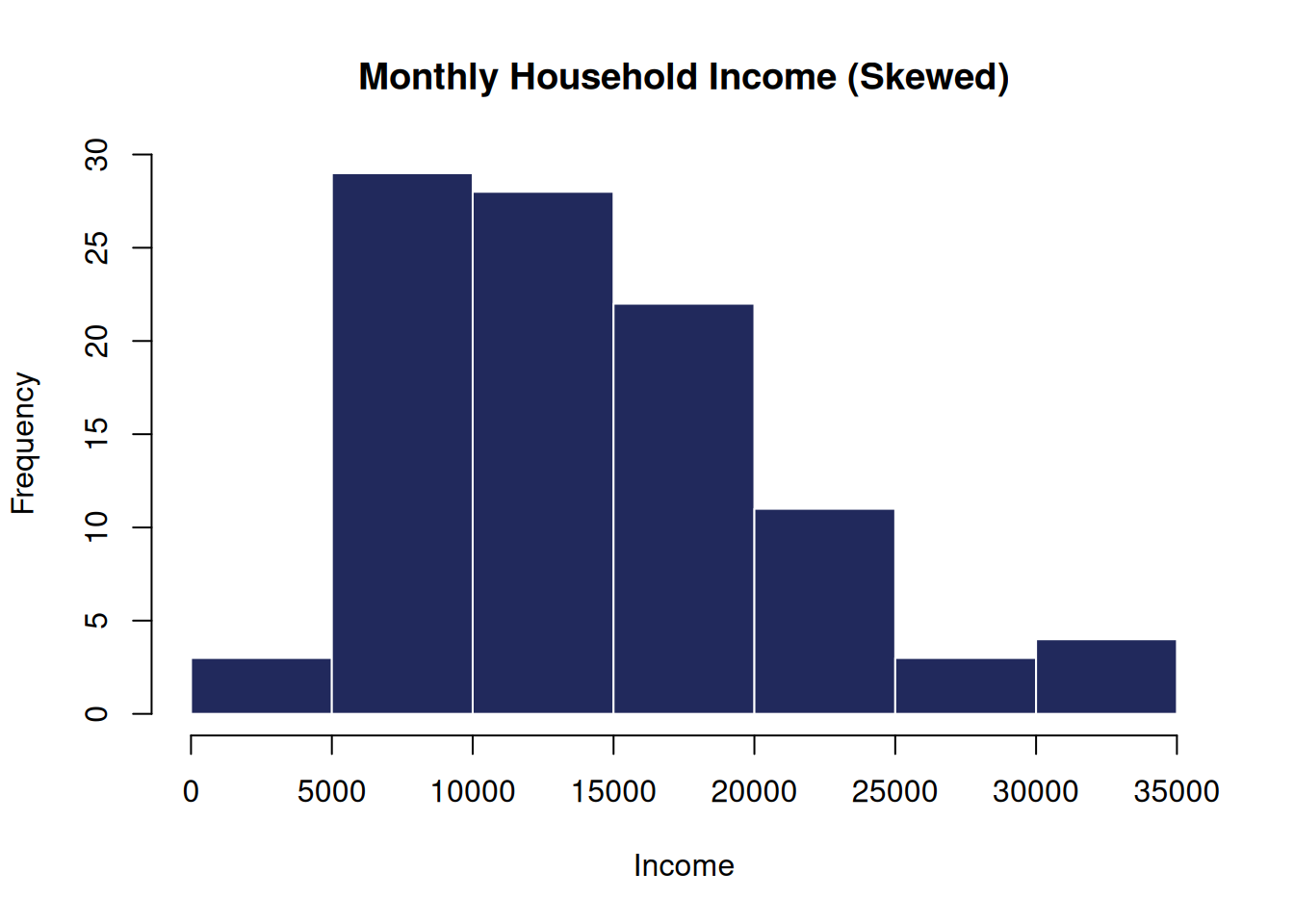
#> [1] 14418.37#> [1] 13381.5Notice the gap between mean and median — a strong sign of skew. A t-based CI for the mean assumes approximate normality of the sampling distribution of the mean; with skewed data and this sample size, that assumption is shakier, and there’s no simple textbook formula at all for some statistics we might want (like the median).
Run t.test(income$monthly_income)$conf.int. Now imagine you wanted a CI for the median income instead of the mean. Try median.test() — it doesn’t exist in base R! This is exactly the gap resampling fills.
3.2 The Logic of Resampling
The core idea: if we can’t derive a sampling distribution mathematically, we can approximate it empirically by treating our one sample as a stand-in for the population, and repeatedly drawing new samples from it, with replacement.
3.2.1 Step 1: Understanding “Sampling with Replacement”
Before resampling our big dataset, let’s look at how R’s sample() function works on a tiny vector of 5 numbers: x <- c(10, 20, 30, 40, 50).
- Sampling WITHOUT Replacement (Shuffling): Every number can only be chosen once.
#> [1] 50 10 40 20 30- Sampling WITH Replacement (Resampling): Each time R picks a number, it “puts it back” into the bag before picking the next one. This means some numbers might appear multiple times, and others might not appear at all!
#> [1] 30 40 40 50 40#> [1] 20 20 30 50 10Notice that in the output, some numbers repeat (e.g., 30 twice) and some are missing. This matches how bootstrapping operates!
3.2.2 Step 2: Drawing ONE Resample of Our Dataset
Now let’s apply this to our income$monthly_income dataset (which contains 100 observations). Let’s draw one bootstrap sample (of the same size, 100, with replacement) and compute its mean:
n <- length(income$monthly_income)
# Draw a resample of size n
one_resample <- sample(income$monthly_income, size = n, replace = TRUE)

# Compare original mean vs resampled mean
mean(income$monthly_income)
#> [1] 14418.37#> [1] 15040.493.2.3 Step 3: Drawing 5 Resamples to Watch the Mean Fluctuate
If we repeat this process 5 times, we get 5 slightly different means:
sapply(1:5, function(i) {
  resample <- sample(income$monthly_income, size = n, replace = TRUE)
  mean(resample)
})
#> [1] 13840.46 13902.35 14971.23 12668.58 14394.38Each resample gives a slightly different mean. The spread of these means across thousands of resamples represents the uncertainty of our original sample mean estimate.
3.3 The Manual Bootstrap Algorithm (Using a Loop)
To build a full sampling distribution, we repeat this process \(B = 2000\) times using a for loop, saving the resampled mean in an empty vector at each step:
# 1. Choose replication size (B = 2000 is standard)
B <- 2000

# 2. Set up an empty vector to store results
boot_means <- numeric(B)

# 3. Run the loop
for (i in 1:B) {
  resample <- sample(income$monthly_income, replace = TRUE)
  boot_means[i] <- mean(resample)
}

# 4. Plot the results!
hist(boot_means,
     main = "Bootstrap Distribution of the Mean",
     xlab = "Resampled Mean Income",
     col = "#065A82",
     border = "white")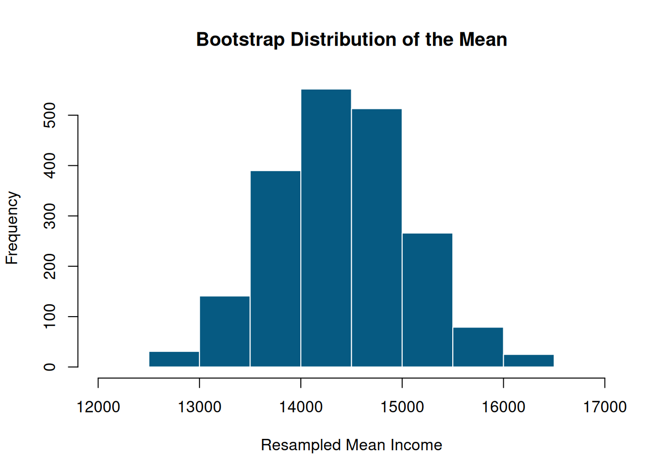
We can now compute the standard error (the standard deviation of our resampled means) and compare it to the original mean:
#> [1] 14410.82#> [1] 667.66593.4 The Professional Workflow: Using the boot Package
While writing a loop is excellent for learning, modern R programmers use the boot package. It is faster and automatically calculates multiple types of confidence intervals.
To use the boot package, we must write a custom function that accepts two arguments:
data: The dataset.indices: A vector of row numbers thatbootgenerates during resampling.
3.4.1 How do “Indices” work? (The Index Mechanics)
Students often find the indices argument confusing. Let’s see what it does in detail:
Imagine your dataset is d <- c("A", "B", "C").
During bootstrap resampling, the boot package generates a random set of row indices, for example: i <- c(1, 1, 3).
Inside our function, R subsets our data using these indices: d[i], which outputs c("A", "A", "C").
Let’s test this manually:
# Let's write a simple mean function that uses index subsetting
mean_fn <- function(data, indices) {
  resampled_subset <- data[indices]
  return(mean(resampled_subset))
}

# Run it manually on the full data using regular indices (1 to 100):
mean_fn(income$monthly_income, 1:100)
#> [1] 14418.37# Run it manually using a set of random resampled indices:
random_indices <- sample(1:100, replace = TRUE)
mean_fn(income$monthly_income, random_indices)#> [1] 14735.64Now that our function works, we pass it to the boot() function, which handles the loop and index generation automatically:
library(boot)

# Run the bootstrap simulation
boot_result <- boot(data = income$monthly_income, statistic = mean_fn, R = 2000)

# Print the boot summary
boot_result
#>
#> ORDINARY NONPARAMETRIC BOOTSTRAP
#>
#>
#> Call:
#> boot(data = income$monthly_income, statistic = mean_fn, R = 2000)
#>
#>
#> Bootstrap Statistics :
#> original bias std. error
#> t1* 14418.37 -10.36739 671.0528Notice: original shows the original sample mean, and std.error shows the bootstrap standard error (matching our manual loop standard deviation).
3.5 Bootstrap Confidence Intervals: Percentile and BCa
Once we run boot(), we can extract the standard error and compute confidence intervals using boot.ci():
#> [1] 671.0528# Calculate both 95% Percentile and BCa Confidence Intervals
boot.ci(boot_result, type = c("perc", "bca"))#> BOOTSTRAP CONFIDENCE INTERVAL CALCULATIONS
#> Based on 2000 bootstrap replicates
#>
#> CALL :
#> boot.ci(boot.out = boot_result, type = c("perc", "bca"))
#>
#> Intervals :
#> Level Percentile BCa
#> 95% (13111, 15758 ) (13199, 15831 )
#> Calculations and Intervals on Original ScaleBias-Corrected and Accelerated (BCa) Confidence Intervals
While the Percentile Bootstrap Interval (obtained via type = "perc") is simple and intuitive, it assumes that the bootstrap distribution is unbiased and has constant variance. If the bootstrap distribution is skewed or has non-constant variance (heteroscedasticity), percentile intervals can fail to provide the nominal coverage (e.g., a “95% interval” might only contain the parameter 91% of the time).
To correct for these limitations, the Bias-Corrected and Accelerated (\(BC_a\)) interval (obtained via type = "bca") introduces two correction factors:
- Bias Correction (\(z_0\)): Corrects for asymmetry in the bootstrap distribution (the extent to which the median of the bootstrap replicates differs from the original sample estimate).
- Acceleration (\(a\)): Corrects for changes in the standard error of the statistic as the parameter value changes (skewness in the sampling distribution).
The \(BC_a\) interval is more computationally intensive and requires larger bootstrap replications (\(R \ge 1000\) or \(2000\)), but it is mathematically superior and preferred for skewed or non-normal data.
Let’s compare these to the classical t-based parametric interval:
#> [1] 13097.04 15739.70
#> attr(,"conf.level")
#> [1] 0.95
Check Before You Run This (Bootstrap Confidence Interval Diagnostics) Before relying on bootstrap confidence intervals, verify these conditions:
- Representative Sample: The sample must be representative of the underlying population. The bootstrap cannot correct for selection bias.
- Independence: The observations must be independent of one another (no clustering or serial correlation).
- Replication Size (\(R\)): Ensure \(R \ge 1000\) (preferably 2000) for stable percentile and \(BC_a\) intervals. Small values of \(R\) lead to highly unstable endpoints.
How to Report This in a Paper: > “The mean monthly household income was estimated to be $14,418.37 (Bootstrap \(SE = \$671.05\)). A 95% bias-corrected and accelerated (\(BC_a\)) bootstrap confidence interval for the mean was [$13,199, $15,831], indicating that the true mean is likely within this range.”
3.5.1 Bootstrapping a statistic with no textbook formula: the median
median_fn <- function(data, indices) median(data[indices])
boot_median <- boot(income$monthly_income, statistic = median_fn, R = 2000)
boot.ci(boot_median, type = c("perc", "bca"))
#> BOOTSTRAP CONFIDENCE INTERVAL CALCULATIONS
#> Based on 2000 bootstrap replicates
#>
#> CALL :
#> boot.ci(boot.out = boot_median, type = c("perc", "bca"))
#>
#> Intervals :
#> Level Percentile BCa
#> 95% (11687, 15155 ) (11561, 14885 )
#> Calculations and Intervals on Original ScaleBootstrapping Variance
In many clinical and scientific studies, we are interested in comparing the variability (variance) of a measurement. Unlike the mean, sample variance does not have a clean, robust parametric confidence interval formula under non-normality. Let’s bootstrap the variance of our skewed income dataset:
var_fn <- function(data, indices) var(data[indices])
boot_var <- boot(income$monthly_income, statistic = var_fn, R = 2000)
boot_var
#>
#> ORDINARY NONPARAMETRIC BOOTSTRAP
#>
#>
#> Call:
#> boot(data = income$monthly_income, statistic = var_fn, R = 2000)
#>
#>
#> Bootstrap Statistics :
#> original bias std. error
#> t1* 44344993 -372290.9 5985341#> BOOTSTRAP CONFIDENCE INTERVAL CALCULATIONS
#> Based on 2000 bootstrap replicates
#>
#> CALL :
#> boot.ci(boot.out = boot_var, type = c("perc", "bca"))
#>
#> Intervals :
#> Level Percentile BCa
#> 95% (32943582, 56292079 ) (34421297, 58907968 )
#> Calculations and Intervals on Original ScaleSecond example — bootstrapping a correlation coefficient, using mtcars:
cor_fn <- function(data, indices) {
  d <- data[indices, ]
  cor(d$hp, d$mpg)
}
boot_cor <- boot(mtcars, statistic = cor_fn, R = 2000)
boot_cor$t0                     # the original correlation
#> [1] -0.7761684#> BOOTSTRAP CONFIDENCE INTERVAL CALCULATIONS
#> Based on 2000 bootstrap replicates
#>
#> CALL :
#> boot.ci(boot.out = boot_cor, type = "perc")
#>
#> Intervals :
#> Level Percentile
#> 95% (-0.8733, -0.6904 )
#> Calculations and Intervals on Original ScaleUsing the course_dataset.csv file (load it with read.csv("data/course_dataset.csv")), bootstrap a 95% CI for the median of baseline_pain. Compare it to a t-based CI for the mean of the same variable — are they telling a similar or different story?
3.6 Bootstrap Confidence Intervals for Proportions
course_df <- read.csv("data/course_dataset.csv")
p_hat <- mean(course_df$response == "Responder")
p_hat
#> [1] 0.7277778Wald CI (parametric, via prop.test):
n_responders <- sum(course_df$response == "Responder")
n_total <- nrow(course_df)
prop.test(n_responders, n_total)$conf.int
#> [1] 0.6555826 0.7900526
#> attr(,"conf.level")
#> [1] 0.95Bootstrap CI:
prop_fn <- function(data, indices) {
  mean(data[indices] == "Responder")
}
boot_prop <- boot(course_df$response, statistic = prop_fn, R = 2000)
boot.ci(boot_prop, type = "perc")
#> BOOTSTRAP CONFIDENCE INTERVAL CALCULATIONS
#> Based on 2000 bootstrap replicates
#>
#> CALL :
#> boot.ci(boot.out = boot_prop, type = "perc")
#>
#> Intervals :
#> Level Percentile
#> 95% ( 0.6611, 0.7944 )
#> Calculations and Intervals on Original ScaleWith a moderate proportion (not extremely close to 0 or 1) and a reasonably large sample (as here, where \(\hat{p} \approx 0.73\)), the Wald and bootstrap intervals usually agree closely. The bootstrap approach earns its keep most clearly when the proportion is close to 0 or 1, or when the sample size is small, situations where the Wald interval can behave badly (even extending below 0% or above 100%, which is nonsensical for a proportion).
Second example — a small, extreme proportion where the two methods diverge more:
set.seed(1)
rare_event <- rbinom(30, size = 1, prob = 0.05)   # only ~5% "successes", small n
mean(rare_event)
#> [1] 0.03333333#> [1] 0.001742467 0.190530216
#> attr(,"conf.level")
#> [1] 0.95#> BOOTSTRAP CONFIDENCE INTERVAL CALCULATIONS
#> Based on 2000 bootstrap replicates
#>
#> CALL :
#> boot.ci(boot.out = boot(rare_event, function(d, i) mean(d[i]),
#> R = 2000), type = "perc")
#>
#> Intervals :
#> Level Percentile
#> 95% ( 0.0, 0.1 )
#> Calculations and Intervals on Original ScaleNotice how much wider and more asymmetric the bootstrap interval looks here — that asymmetry is real information the symmetric Wald interval simply cannot represent.
3.7 An End-to-End Bootstrap Workflow
Here’s a repeatable process you can apply to any new dataset:
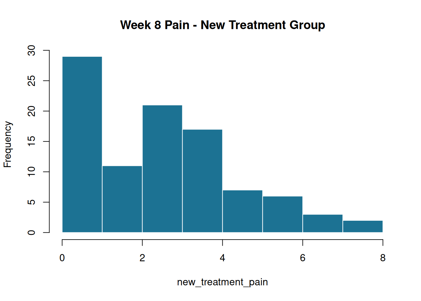
# STEP 1: State the question
# "What is the mean week-8 pain score for patients on the New treatment?"

# STEP 2: Check assumptions
new_treatment_pain <- course_df$week8_pain[course_df$treatment == "New"]
hist(
  new_treatment_pain,
  main = "Week 8 Pain - New Treatment Group",
  col = "#1C7293", border = "white"
)
#>
#>  Shapiro-Wilk normality test
#>
#> data:  new_treatment_pain
#> W = 0.94252, p-value = 0.0003735
# STEP 3: Run the bootstrap
mean_fn2 <- function(data, indices) mean(data[indices])
boot_final <- boot(new_treatment_pain, statistic = mean_fn2, R = 2000)
# STEP 4: Construct the CI
ci_final <- boot.ci(boot_final, type = "perc")
ci_final#> BOOTSTRAP CONFIDENCE INTERVAL CALCULATIONS
#> Based on 2000 bootstrap replicates
#>
#> CALL :
#> boot.ci(boot.out = boot_final, type = "perc")
#>
#> Intervals :
#> Level Percentile
#> 95% ( 2.083, 2.828 )
#> Calculations and Intervals on Original Scale# STEP 5: Report
cat(sprintf(
paste0(
"Mean week-8 pain in the New treatment group: %.2f ",
"(95%% bootstrap CI: %.2f to %.2f)\n"
),
mean(new_treatment_pain),
ci_final$percent[4],
ci_final$percent[5]
))#> Mean week-8 pain in the New treatment group: 2.45 (95% bootstrap CI: 2.08 to 2.83)Repeat this exact five-step workflow, but for the Standard treatment group instead of New. Do the two confidence intervals overlap? What would that suggest about the two treatments?
- Parametric CIs rely on assumptions (usually approximate normality) that skewed or small data can violate.
- The bootstrap approximates a sampling distribution empirically, by resampling your data with replacement many times.
boot()+boot.ci()is the standard R workflow — and it generalizes to any statistic, even ones with no textbook CI formula (medians, correlations, custom metrics).- Bootstrap CIs for proportions are especially valuable when the sample is small or the proportion is near 0 or 1.
- A repeatable five-step workflow (question → check assumptions → bootstrap → CI → report) will serve you for the rest of this course and beyond.
Next, in Chapter 4, we move from continuous variables to categorical data — contingency tables, agreement measures, and the art of reporting them compactly.
Chapter 3 covered:
- Correct interpretation: A 95% CI does not mean “95% probability the parameter is in this interval” — it means 95% of intervals constructed this way, over repeated samples, would contain the true parameter
- Parametric CIs: Based on the \(t\)-distribution (mean), normal approximation (proportion), and their differences — require distributional assumptions
- Bootstrap principle: Treat the sample as a proxy for the population; resample with replacement \(B\) times; the variability of the bootstrap statistic estimates the sampling variability
- Bootstrap CI types: Percentile (simple), Basic (bias-corrected), BCa (bias-corrected and accelerated — most accurate)
- When to bootstrap: Small samples, unknown distributions, complex estimators (correlation, ratio, regression coefficients)
| Method | Formula | When to Use |
|---|---|---|
| One-sample \(t\) | \(\bar{x} \pm t_{n-1, \alpha/2} \cdot s/\sqrt{n}\) | Normal population or \(n \geq 30\) |
| Proportion (Wald) | \(\hat{p} \pm z_{\alpha/2}\sqrt{\hat{p}(1-\hat{p})/n}\) | \(n\hat{p} \geq 10\), \(n(1-\hat{p}) \geq 10\) |
| Bootstrap (percentile) | \([\hat\theta^*_{(B\alpha/2)},\, \hat\theta^*_{(B(1-\alpha/2))}]\) | Any estimator, any distribution |
Coming up: Chapter 4 moves from continuous outcomes to categorical data — contingency tables, association tests, and agreement measures.
3.8 Lab 3: Confidence Intervals for the Course Dataset
Objective: Construct and compare parametric and bootstrap CIs for multiple estimands from the course_dataset.
Dataset: course_dataset.csv
3.8.2 Step 2: Parametric CI for Mean Baseline Pain
# Using t.test (returns CI automatically)
t_result <- t.test(course_df$baseline_pain, conf.level = 0.95)
cat("95% CI for mean baseline pain:
")
#> 95% CI for mean baseline pain:#> 5.97 6.583.8.3 Step 3: CI for Proportion of Responders
n_resp <- sum(course_df$response == "Responder")
n_total <- nrow(course_df)
# Wilson CI (more accurate than Wald for proportions)
prop.test(n_resp, n_total, conf.level = 0.95)
#>
#> 1-sample proportions test with continuity correction
#>
#> data: n_resp out of n_total, null probability 0.5
#> X-squared = 36.45, df = 1, p-value = 1.566e-09
#> alternative hypothesis: true p is not equal to 0.5
#> 95 percent confidence interval:
#> 0.6555826 0.7900526
#> sample estimates:
#> p
#> 0.72777783.8.4 Step 4: Bootstrap CI for the Median
set.seed(42)
median_fn <- function(data, indices) median(data[indices])
boot_out <- boot(course_df$baseline_pain, statistic = median_fn, R = 2000)
boot.ci(boot_out, type = c("perc", "basic"), conf = 0.95)
#> BOOTSTRAP CONFIDENCE INTERVAL CALCULATIONS
#> Based on 2000 bootstrap replicates
#>
#> CALL :
#> boot.ci(boot.out = boot_out, conf = 0.95, type = c("perc", "basic"))
#>
#> Intervals :
#> Level Basic Percentile
#> 95% ( 6.0, 6.9 ) ( 5.7, 6.6 )
#> Calculations and Intervals on Original Scale3.8.5 Step 5: Bootstrap CI for the Difference in Means (New vs Standard Treatment)
set.seed(42)
diff_fn <- function(data, indices) {
  d <- data[indices, ]
  mean(d$baseline_pain[d$treatment == "New"], na.rm = TRUE) -
  mean(d$baseline_pain[d$treatment == "Standard"], na.rm = TRUE)
}
boot_diff <- boot(course_df, statistic = diff_fn, R = 2000, strata = as.factor(course_df$treatment))
boot.ci(boot_diff, type = c("perc", "norm", "basic"), conf = 0.95)
#> BOOTSTRAP CONFIDENCE INTERVAL CALCULATIONS
#> Based on 2000 bootstrap replicates
#>
#> CALL :
#> boot.ci(boot.out = boot_diff, conf = 0.95, type = c("perc", "norm",
#> "basic"))
#>
#> Intervals :
#> Level Normal Basic Percentile
#> 95% (-0.7911, 0.4238 ) (-0.7949, 0.4164 ) (-0.7801, 0.4312 )
#> Calculations and Intervals on Original Scale3.8.6 Lab Exercises
- Compute a 90% and 99% t-interval for mean
week8_pain. How do they differ in width? - Compute bootstrap CIs for the correlation between
baseline_painandweek8_painusingR = 1000resamples. - Compare the parametric and bootstrap 95% CI for the mean of
baseline_pain. Are they similar? If they differ, what might explain the difference?